Calibrating the XtaLAB Synergy-S for PDF Analysis
Introduction
Pair Distribution Function (PDF) Analysis¹ has become a versatile tool for understanding the structure, and ultimately properties, of materials. Under normal circumstances, PDF is a technique performed using powdered samples and on suitable powder diffractometers. Modern microfocus singlecrystal diffractometers contain exceptionally bright sources and feature ultralow-noise HPC detectors that make them capable of performing high-quality diffraction experiments on microgram quantities of powder. A natural extension of these features is to perform PDF experiments on such equipment.
The most popular tool for the refinement of structures using PDF data is PDFgui². In order to bootstrap refinement of a structure using PDFGui, it is important to have reasonable starting values for the unit cell parameters, and the parameters
Qdamp and Qbroad. The unit cell parameters can be determined using whole powder pattern fitting (WPPF), but Qbroad and Qdamp must be determined for your experimental setup.
As a review, the data against which the atomic model is refined in PDFGui is the reduced pair distribution function, G(r). This function is the Fourier transform of Q(S(Q)-1), which is directly derived from the raw data.
Given an atomic level model, the calculated reduced PDF, $G_c(r)$, can be expressed as:
$G_c(r) = \frac{1}{r}\sum_i\sum_j[(\frac{f_if_j}{\langle f^2 \rangle})\delta(r-r_{ij})] - 4\pi r\rho_0$
where $f_{i,j}$ is the scattering factor of atom i or j, ⟨f⟩ is the scattering factor averaged over all atoms in the model, $r_{ij}$ is the distance between atoms atom i and j, and $\rho_0$ is the number density. The sum is over all atom pairs in the unit cell. For distances between r = 0 and the separation of the first atom pair, the function will have a slope of $-4 \pi r \rho_0$. Qbroad is a correction for broadening from increased noise at high Q (Å⁻¹). Qbroad also encompasses traditional microstrain contributions from a powder sample.
Qbroad modifies the $G_c(r)$ peak width as shown below:
$\sigma\prime_{ij}=\sigma_{ij}\sqrt{1-\frac{\delta_1}{r_{ij}}-\frac{\delta^2_2}{r^2_{ij}}+Q^2_{broad}r^2_ij}$
Where $\sigma_{ij}$ is the peak width without correlation and is computed from the anisotropic displacement parameters. $\delta_1$ and $\delta_2$ account for correlated motion at different temperatures. Discussion of these two terms is outside the scope of this document. The effect of Qbroad is shown in Figure 1. Note how the peaks at larger values of r become broader and weaker as Qbroad increases.
Qdamp applies a Gaussian dampening envelope arising from limited Q-resolution (Å⁻¹) to the reduced PDF. Figure 2 displays the consequences of increasing Qdamp on G(r).
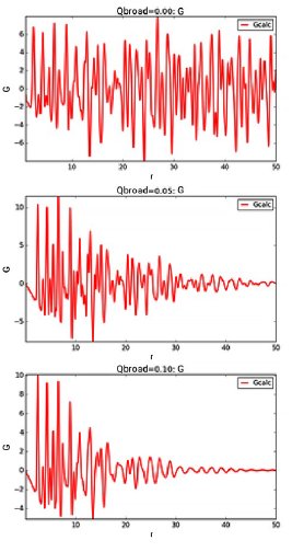
Figure 1: Effect of Qbroad on the calculated G(r) for nickel powder.
$B(r)=e^{\frac{-(rQ_{damp})^2}{2}}$
Note the effect of Qbroad on the reduced PDF vis-à-vis Qdamp. Qdamp causes the G(r) function to fall rapidly, but the peak widths remain the same. Qdamp encompasses traditional crystal size contributions from a powder sample and also allows for change in instrument peak width with change in X-ray wavelength.
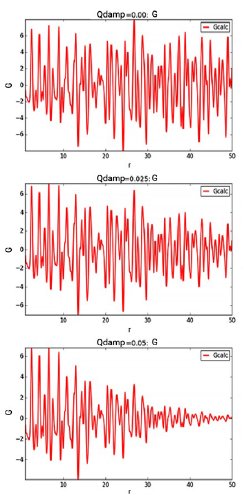
Figure 2: Effect of increasing Qdamp on the reduced PDF.
Experimental
For this procedure, we prepared nickel powder with a trace amount of oil in a MiTeGen³ loop as the reference standard, see Figure 3. Images for both the nickel and the background (loop and instrument) were collected on a XtaLAB Synergy-S with molybdenum radiation and a HyPix-6000HE.
The beam size at the sample is approximately 100 μm and the divergence is 4 mR. The data were collected at a sample-to-detector distance of 32 mm using a single axis scan. At this distance, a 100 μm pixel subtends an angle of approximately 0.18°. Figure 4 displays a representative diffraction image from the nickel powder sample. The images were converted to 2θ vs I data using CrysAlisPro using the appropriate Lorentz and polarization corrections. We assumed the sample was spherical around the scan axis and, thus, no absorption correction was applied.
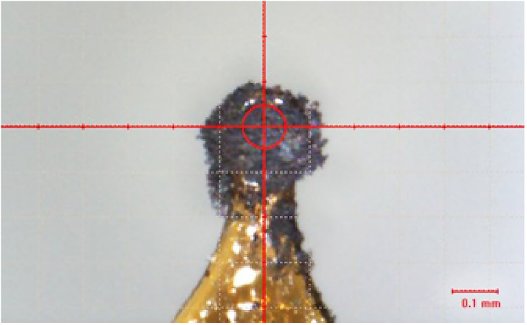
Figure 3: Nickel powder mounted on a MiTeGen loop held together with a trace of oil
The reduced G(r) was generated from the nickel and sample holder/instrument background 2𝜃 vs I data using SmartLab Studio II using the defaults in the PDF plugin with the exception of increasing the output range from 10 Å to 50 Å.
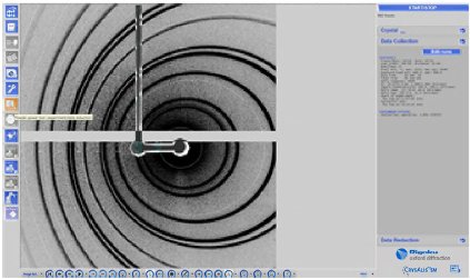
Figure 4: Representative diffraction image for nickel powder
Refinement of the model against the reduced PDF was performed with PDFGui using the CIF for Ni from the Crystallographic Open Database. In order to prevent singularities, refinement began with the scale factor and unit cell parameter, then adding the ADP, Qdamp, Qbroad and $\delta_2$ individually until convergence one pass at a time.
The step-by-step details of the processing may be learned in the video at the Rigaku X-ray Forum.
Results
The results of the refinement are displayed in TABLE 1 and Figure 5. Figure 5 shows a good fit between the G(r) data from SmartLab Studio II (blue open circles). The refined parameters are scale factor = 1.096(13), Qdamp = 0.0311(6) Å, = Qbroad = 0.018(1) Å⁻², δ₂ = 1.5(2), a = b = c = 3.52457(15) Å, and U11= U22= U33 = 0.009998(18) Å⁻² with a reduced χ² value of 0.124 and Rw = 0.0999.
The values of reduced χ² value and Rw indicate a reasonably good fit between the observed and calculated G(r) functions. Thus, the values of Qdamp and Qbroad can be used as a starting point for refinement of other similar samples measured using the same instrument configuration.
Table 1: PDFGui refinement results for nickel powder
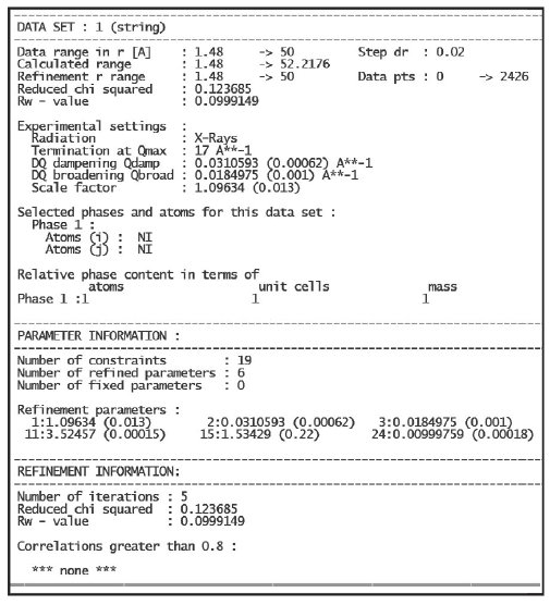
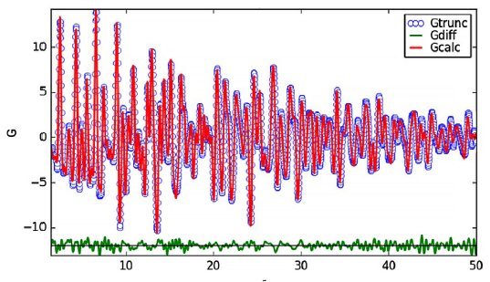
Figure 5: Observed versus calculated G(r) function. Observed data are blue circles, calculated data is the red line and the residual is the green curve
Conclusions
We have shown the process by which one can calibrate a XtaLAB Synergy system for PDF use. It is important to remember that the calibration data should be collected under the same conditions as you might collect the data on an unknown; that is, using the same wavelength, sample-to-detector distance, etc.
References
- Underneath the Bragg Peaks: Structural Analysis of Complex Materials, 2nd Ed, by T. Egami and S. J. L. Billinge, Elsevier, Amsterdam, 2012.
- C L Farrow, P Juhas, J W Liu, D Bryndin, E S Božin, J Bloch, Th Proffen and S J L Billinge 2007 J. Phys.: Condens. Matter 19 335219
- MiTeGen, LLC, P.O. Box 3867, Ithaca, NY 14852 software.

Contact Us
Whether you're interested in getting a quote, want a demo, need technical support, or simply have a question, we're here to help.